A simple linear regression using MCMC

Bayesian framework

Let us assume we have a problem to solve. Before collecting any data we have some prior beliefs about the problem. We then collect some data for solving the problem. In Bayesian approach, we will combine our prior beliefs with data collected to form new posterior beliefs about the problem.

Markov Chain Monte Carlo (MCMC) methods do not calculate the exact form of posterior distribution,  but instead simulate draws from it. Generally speaking, the methods are run for many iteration and at each iteration an estimate for each unknown parameter is produced. The estimates from the last iteration are used to produce new estimates. The methods are to generate a sample of values from the posterior distribution of the unknown parameters we studied.

Let us consider a simple linear regression model as an example

where  and  are the fixed and random parameters. A joint posterior distribution, , is produced for the above parameters that combines the prior information with the data.

MCMC estimation

In the simple linear regression model, we would like to generate samples from the posterior distribution  with three unknowns. The joint posterior distribution is difficult to simulate from, but the conditional posterior distributions can be simulated from easily. This is due to the fact that sampling from these conditional posterior distributions in turn is equivalent to sampling from the joint posterior distribution.

Gibbs sampling algorithm

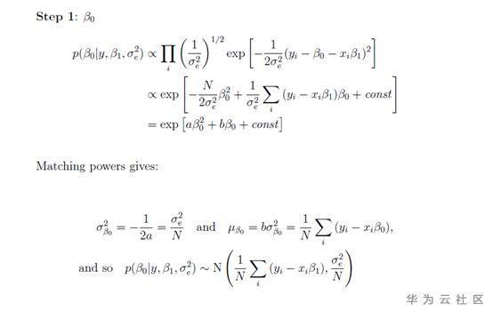
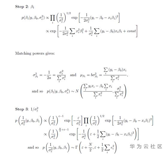
Let us assume the non-informative priors,  where    We work with the precision parameter,  rather than the variance, . Then our posterior distributions can be calculated as follow:

Metropolis Hastings algorithm

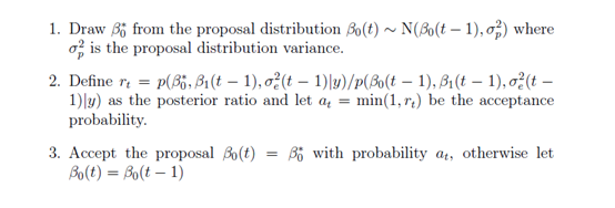
If the conditional distributions do not have the simple form, then Metropolis Hastings sampling will be considered. In general MCMC methods generate new values from a proposal distribution that determines how to choose a new parameter value given the current one. The proposal distribution suggests a new value for the parameter of interest. This new value is then either accepted  as the new estimate for the next iteration or rejected and the current value is used as the new estimate for the next iteration.

In our example, the updating procedure for the parameter  at time  as follows:

Reference

MCMC Estimation in MLwiN, v3.03 (PDF, 6,430kB).  Browne, W.J. (2019) Centre for Multilevel Modelling, University of Bristol

Appendix

R code for the tutorial data set: http://www.bristol.ac.uk/cmm/media/r2mlwin/MCMCGuide01.Rout